On computing next greater intervals in linear time

Recently, a close friend convinced me to start solving problems from online judges. While I don’t have the slightest intention of competing in contests, I couldn’t refuse the reason for solving interesting problems. In the initial phases, I came across a few problems that required computation of nextGreaterInterval for every element of a given $list$ in linear time. The most popular (and efficient) method to solve this problem is to use a monotonic stack. While one can find plenty of implementation and problem specific resources on the web, none does enough justice to the elegant usage of the data structure, its design and its characteristic generalization property. Using monotonic stack over a brute force solution prunes the search space from a quadratic function of input size to a linear function $i.e. O(N^{2}) \, –> O(N)$.

I was compelled to present my notes on this topic owing to the fact above. Thus, my treatment will be generic, (somewhat) formal and design oriented. Since I had spent a fair amount of time hacking my brains to understand the machinery the first time I saw it, I try to build a lucid understanding by reverse engineering the data structure one step at a time.

I assume that the reader is familiar with very basics of algorithmic analysis (or counting), some Python (or English) and some set notation. There’s still something for you even if you don’t have a background in any of the above.

Problem statement

Let’s start by setting up our problem in a simplistic notation, read Pythonic pseudo code. For the sake of simplicity, assume that we have a random access $list$ of distinct non-negative integers. $N$ is the length of $list$ and $list[i] \, : 0 < i < N$ is the $i$th element of $list$.

P: We need to find the nextGreaterInterval with respect to an element $list[i]$ is defined as $[leftBound, rightBound]$, such that:

• $leftBound = list[x] : list[x] > list[i], \, x < i \, and \, list[i] >= list[k] \, \forall k \in [x+1, i-1]$
• $rightBound = list[y] : list[y] > list[i], \, y > i \, and \, list[i] >= list[k] \, \forall k \in [i+1, y-1]$

Let’s say we have separate lists leftBound and rightBound such that the $leftBound[i]$ is the index of the left bound of $list[i]$ and $rightBound[i]$ is the index of the right bound respectively. If an element $list[i]$ doesn’t have a sound left bound then we set $leftBound[i]$ to $-1$; similarly we set $rightBound[i]$ to $N$.

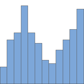
For example, in the image above nextGreaterInterval for element $list[5]$ is $[4, 9]$ and that for $list[4]$ is $[3, 10]$

Motivation for the problem

Many programming problems can be reduced to P. Hence the solution to P can be used as a sub-routine in the solution of original problem. I’ll illustrate a well-known problem to motivate the development of a solution to P.

Check out this problem from spoj. After a few preliminary sanity checks, you can convince yourself that every entry in the histogram forms a rectangle in its nextLesserInterval. The nextLesserInterval is just nextGreaterInterval with respect to the $<$ operator. Hence each such rectangle will be a candidate for max-area rectangle. Thus, this problem can be easily solved once we have a solution for P.

Designing the machinery

It typically helps to solve a simpler version of the original problem to get started. More complexity can be added step-by-step to reach the solution for the original problem. Hence, I first consider the problem for computing $leftBound$ separately.

Computing the leftBound list

A naive way to compute left bound for an element $list[i]$ is to linearly search leftward in $list$ till you find the first element greater than $list[i]$. In the worst case there are $i$ states to check for every element $list[i]$, leading to a total of $O(N^{2})$ states. Thus it’ll take $O(N^{2})$ time to compute the $leftBound$ list.

However, say we already have $leftBound$ computed for the first $i$ elements of $list$. For $i+1$th element, let’s call it $curr$ we have two cases:

• Case1 : $curr < list[i]$
  • In this case $list[i]$ will trivially be the left bound of $curr$.
• Case2 : $curr >= list[i]$
  • Here we can use the naive way of searching linearly leftwards in $list$ till we find the first element greater than $curr$. However there’s a catch here; observe that from the definition of $leftBound$, one can notice that the elements between $list[leftBound[i]]$ and $list[i]$ are smaller than $list[i]$. Hence they must be smaller than $curr$ too.
  • Thus instead of searching linearly leftwards, we could skip the elements in between and directly check $list[leftBound[i]]$, then $list[leftBound[leftBound[i]]]$ and so on until we find the first element greater than $curr$.
  • The set of indices $i$, $leftBound[i]$, $leftBound[leftBound[i]]$ and so on form a topology of ancestors dictated strictly by the ordering with respect to $>$ operator. At this point we can safely conclude that computation of left bound for a new element depends only on the topological ancestors of the last seen element in the $list$.

Hence we have pruned the search space but by how much? We will discuss the answer to this shortly.

The monotonic stack

There are two noteworthy observations to make considering that we need only maintain the topological ancestors of the last element in the $list$ to compute the left bound of $curr$:

• Case1 tells us that $curr$ can simply be added to the front of the topology without disturbing the rest of its structure. Case2 tells us that once we find the left bound of $curr$, we don’t need to maintain any elements between $curr$ and its left bound. If you stare at the screen long enough, you’ll notice that Case1 and Case2 together manifest a last-in-first-out behaviour in the topology of ancestors. Hence a stack can be used to represent the topological ancestors of the last element in $list$.
• Case2 also suggests that the topology obeys the following invariant $ancestor(item) > item \, \forall item \in topology$. The invariant is equivalent to monotonicity in the stack.

Thus monotonic stack gets its name from the two observations made above. So far so good! Now we are in a position to write down the semantics of the proposed data structure. I am (again) choosing Pythonic code to write the semantics.

class MonotonicStack(Stack):

    @abstractmethod
    def is_empty():
        """Returns true if the topology doesn't contain any elements, false otherwise"""
        raise NotImplementedError

    @abstractmethod
    def push(idx):
        """Adds idx to top of the topology"""
        raise NotImplementedError
    
    @abstractmethod
    def pop():
        """Removes an element from the top of the topology"""
        raise NotImplementedError
    
    @abstractmethod
    def top():
        """Returns the element at the top of the topology"""
        raise NotImplementedError

Let’s try to write an algorithm to compute the left bound for every element in the list using the observations and specified semantics.

topo = MonotonicStack()
for i, item in enumerate(list):
    while not topo.is_empty() and list[topo.top()] < item:
        topo.pop()
    leftBound[i] = -1 if topo.is_empty() else topo.top()
    topo.push(i)

Analyzing the algorithmic complexity and reduction in search space

So now we have an algorithm in place for maintaining the left bounds of elements in a list. Let’s analyze the time and space complexity of this algorithm. The number of operations in the specified algorithm are proportional to the number push and pop calls. Since every element gets pushed and popped out of stack exactly once, we get a total of $2N$ push or pop calls combined. Thus the time complexity of this algorithm is $O(N)$. Since the size of the utility stack can go upto a maximum of $N$, the space complexity is also $O(N)$.

Answering the question of ‘how much of the search space have we pruned?’, we have pruned the search space from $O(N^{2})$ to $O(N)$.

Ok, but what about the rightBound?

Consider the pop calls in the specified algorithm along with the element that is popped out. Clearly its left bound will be the result of the top call but what is its right bound? Are you ready for the revelation? Hold tight onto your chairs and breathe deeply because this is going to blow your mind:
.
.
.
.
item

By the condition on item in the algorithm, the execution will reach the pop call if and only if the invariant list[topo.top()] < item is satisfied. (assume that the stack is not empty in this case, otherwise the right bound index is N)

And we’re done. The left bound of the popped element is the result of the top call while the right bound is item. Since we know the left bound and right bound of an item when it is popped, it is best if we perform any visit(element, leftBound, rightBound) operations at this point. [NOTE: With appropriate design choice, one can write the visit routine with the given signature. : END OF NOTE]

Final algorithm

topo = MonotonicStack()
for i, item in enumerate(list):
    while not topo.is_empty() and list[topo.top()] < item:
        element = topo.top()
        topo.pop()
        leftBound = -1 if topo.is_empty() else topo.top()
        rightBound = i
        visit(element, leftBound, rightBound)
    topo.push(i)

while not topo.is_empty():
    element = topo.top()
    topo.pop()
    leftBound = -1 if topo.is_empty() else topo.top()
    rightBound = len(list)
    visit(element, leftBound, rightBound)

Generalization

We saw in the discussion so far how the $>$ operator dicatates the ancestry topology for every element. The idea of the topology easily extends to $<$ operator. What’s more? It works out just as elegantly for any binary associative comparison operator used to compare records. As long as your operator can decide an ordering between any two records unambiguosly, we will be able the compute the $nextGreaterInterval$ for every element in linear time.

Example problems

The solution to this well-known problem uses the monotonic stack is that of finding the largest rectangle in a histogram. The key idea here is to maintain the $nextGreaterInterval$ with respect to the $<$ operator. visit operation computes the area of the rectangle using the height of the popped out element and its $nextGreaterInterval$ and updates the max value of rectangle.

Here’s another problem that can be solved using the idea of monotonic stack that we just developed. I’ll leave this as an exercise for the reader to figure out the specifics.

Concluding Remarks

Even though the concept is simple, I have seen people, including myself, struggling with understanding of the machinery. Typically we find interesting connections when we reverse engineer the known solution from the atomics. In case of algorithmic design the atomics turn out to be a handul of invariants in the behaviour of the machinery. Be on the lookout for these invariants.

If you find any errors that require corrections raise an issue in this repo. If you find any more relevant references, ideas that I might have missed or the need for me to add illustrative diagrams then feel free to drop me a mail (attach the diagrams to be added in your mail).

References

• A short answer from stackoverflow
• An implementation specific post by labuladong